
If you’re planning a road trip across NSW, there are over 800 official rest areas. But are there enough?
This post identifies sections of highway more than 2 hours from a rest stop. We use a local version of OpenRouteService, an extract from OpenStreetMap maps, and rest area data from Transport for NSW to determine where there are gaps in the Rest Area network.
Rest Stop Points Data
Save a copy of the GEOJSON rest stops:
- Open https://rms-apps.carto.com/api/v2/sql?q=SELECT * FROM ra_get_rest_area_data()&format=GeoJSON”
- Save cartodb-query.json as rest-stops.geojson
- Go to Layer > Add Vector Layer
- Locate rest-stops.geojson
- Accept other defaults
- Click Add
- Click Close
To add the rest stops to QGIS:
- Go to Layer > Add Vector Layer
- Change source type to Directory
- Change type to OpenFileGDB
- Select the folder expanded above
- Click Add
- Click OK on the Vector Layers dialog
- Click Close
The Rest Stops dataset contains both permanent Rest Stops and also Driver Revivers that operate at peak periods. The number of Driver Revivers in the dataset possibly changes depending on when the data was extracted. In the extract used in this study, there were only 15 or so temporary Driver Revivers, which may have been out of date.
For the purpose of this demo, we will assume all stops are active.
Highways Data
Get major highways from NSW Data Portal. Instructions at https://opendata.transport.nsw.gov.au/dataset/road-segment-data-from-datansw
- The file is about 57MB.
- When the email arrives, save the data in the link to your local study area directory
- Expand the .zip file and a new folder for RoadNameExtent_EPSG4283.gdb is created.
To add the road network to QGIS:
- Go to Layer > Add Vector Layer
- Change source type to Directory
- Change type to OpenFileGDB
- Select the folder expanded above
- Click Add
- Click Close
The RoadNameSegment database has many MultiLineStrings. Many tools struggle with multi-lines, so let’s separate them into single parts.
- Open the Processing Toolbox, and search for Multipart
- Double click on the result for Multipart to singleparts
- Set Input Layers as RoadNameExtent_EPSG4283 RoadNameExtent
- Click Run, then Close
A new layer called Single Parts is added. Rename this to NSW Roads. There are about 117,000 segments.
For this study, we’re only interested in the major roads. These have a “functionhierarchy“ of less than or equal to 3:
- Freeways and Motorways are 1
- Highways such as Princes Highway are 2
- Major arterials such as Epping Road are 3
To filter only the roads we need:
- Right-click the NSW Roads layer in the Layers panel and choose Filter…
- Double-click on functionhierarchy, then click <= button, and type the number 3
- Click OK
Isochrones with OpenRouteService
The assumption for this study is that rest stops need to be no more than 2 hours apart on major routes.
So we will create drive time isochrones for the rest stops data.
There is a plugin for QGIS that allows us to create drive times. The plugin is called ORS Tools.
To install this plugin:
- Go to Plugins
- Search for ORS Tools
- Click Install Plugin
- Click Close
The ORS Tools plugins connects to the OpenRoutingService which offers a free API to calculate drive times. However, there are restrictions on the service in order to keep it free. One of the main restrictions is that the maximum range is 60 minutes, and the maximum distance is 120km. If we want 2-hour isochrones, then we need to find an alternative!
Install ORS
ORS can be installed in a Docker container locally, and tweaked as required.
The instructions are at https://giscience.github.io/openrouteservice/installation/Installation-and-Usage.html
The details won’t be covered here – it is very technical and depends on many inputs – operating system, CORS, Docker installs, port settings, URL parameters, OpenStreetMap extracts and more. There will be a separate blog post covering the topic. Whilst it may be a stumbling block for many, perhaps getting the theory is a good start.
When the service is up and running, it can be added as a server in the ORS configuration.
- Click the ORS Tools icon (a black hexagon with red nodes)
- Click on the gear icon
- Click the Add button
- Leave the API key blank (unless you configured it in the local install)
- In the Base URL, enter http://localhost:8080/ors
When the service was installed, a folder called conf was created. Inside that directory is a settings file called ord-config.json.
- Locate the isochrones tree
- For the maximum_range_time, change the default value of 3600 to 7200. These are seconds.
- Restart the Docker container and we’re ready to go.
Create Isochrones
- Open the ORS Tools by clicking on the ORS icon
- Change to Batch Jobs
- Choose Isochrones From Layer
- Change the Provider to your newly added local ORS Service
- Set Input Layer as rest-stops
- Leave travel Mode as driving-car
- Leave Dimension as time
- Change the Comma-Separated ranges to 120 min (which is the same as 7200 seconds)
- Click Run
Features with no ID may cause a GenericServerError. These may or may not be important? I suspect they are records that are too far from the road network to snap to it.
What is happening is the ORS tool is travelling 2 hours in every direction from every rest point and merging those polygons into one layer.
With over 800 rest stops, that is a lot of calculations! By running locally we don’t impact any other users, nor do we consume credits as we might with other network analysis tools.
For this study, the process took 12 minutes.
A new layer called Isochrones is added to the Layers panel.
- Click Close, and Close the ORS Tools dialog.
There are a lot of overlapping isochrones. Your computer may be pleading for mercy at this point as it tries to redraw the map layers.
It makes sense to merge this all into one isochrone since we’re only interested in sections of highway not within 2 hours of any rest stop.
- Open the Processing Toolbox
- Search for Dissolve
- Double click on Vector geometry > Dissolve
- Leave/change the Input layer to be Isochrones
- Click the Spanner icon of the Input Layer
- Change Invalid feature filtering to Skip (ignore) Features with Invalid Geometries
- Click the blue triangle to return to Parameters
- Click Run
This process took about 2 minutes. A new layer called Dissolved was added to the Layers panel.
The Dissolved layer is very complex. We’re going to split it up into tiles to achieve performance improvements.
Create a grid of 100km by 100km squares:
- Go to Vector > Research Tools > Create grid
- Grid type is Polygons
- Grid extent is Calculate From Layer > Dissolved
- Set Horizontal Spacing and Vertical Spacing to 100000m (100 km)
- Click Close
A new layer called Grid is dded to the Layers panel.
To intersect the Grid and the Dissolved layers:
- Search for Intersect in the Processing Toolbox
- Double-click on Vector overlay > Intersection
- Set the Input layer as Dissolved
- Set the Overlay layer as Grid
- Click Run, and when complete click Close
A new layer called Intersection is added to the Layers panel.
- Hide the Grid, Dissolved, and Isochrones layers, and watch performance go back up.
Finding Orphan Highways
We now have all the components we need to calculate sections of highway not within 2 hours of a rest stop.
The algorithm we need is called Difference. The Difference algorithm identifies all parts of the line layer that do not fall within the polygon layer. This is very different to the Split With Lines algorithm which outputs the opposite of what we’re trying to achieve.
- Search for Difference in the processing Toolbox
- Double-click on the Vector overlay > Difference
- Set the Input layer to NSW Roads
- Set the Overlay layer to Intersection
- Click Run
A new layer called Difference is added to the Layers panel.
To see where the orphaned segments are:
- Right-click on Difference and choose Zoom to Layer(s)
- Hide the Intersection layer
- Change the styling for Difference so it really stands out by changing the line thickness to 3 in the Layer Styling panel.
Results
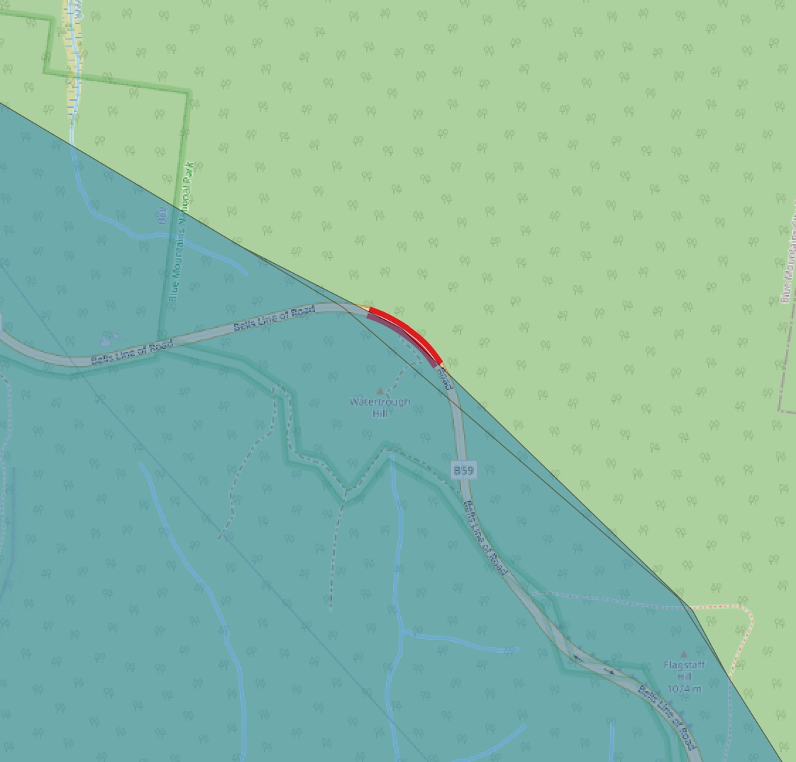
There will be anomalies on the map, and these will usually be caused by either missing data in the OpenStreetMap data or artefacts in the polygon generated by ORS.
For example, there is a highway segment on Bells Line of Road at Bell that turns out to be overlap issue. It is only 150m long.
We’re really only interested in the longest sections of road. Before we can look at the longest sections, we need to split MultiLineStrings into Single LineStrings.
- Search for Multipart in the Processing Toolbox
- Double-click on Multipart to Singleparts
- Choose Difference as the Input Layer
A new layer called Single parts is added to the Layers panel.
We’re going to add a new virtual field for the length of each object:
- Select the Difference layer in the Layers panel
- Open the Field Calculator from the toolbar (abacus)
- Check the Create virtual field
- Name the virtual field as “segment_length” without the quotes.
- Set the Expression to
$length - Click OK
Consider sections of highway that are more than 20 kilometres long:
- Right-click on Single parts in the Layers panel
- Choose Filter…
- Double-click on segment_length at the bottom of the list of Fields
- Add the greater than operator (>), and 20000 as the value:
"segment_length" > 20000
Zoom the map to show all filtered Single parts.
To use the same styling from the Difference layer, perform the following:
- Right-click the Difference layer
- Go to Styles… > Copy Style > All Style Categories
- Right-click on the Single parts layer
- Go to Styles… > Paste Style > All Style Categories
- Hide the Difference layer
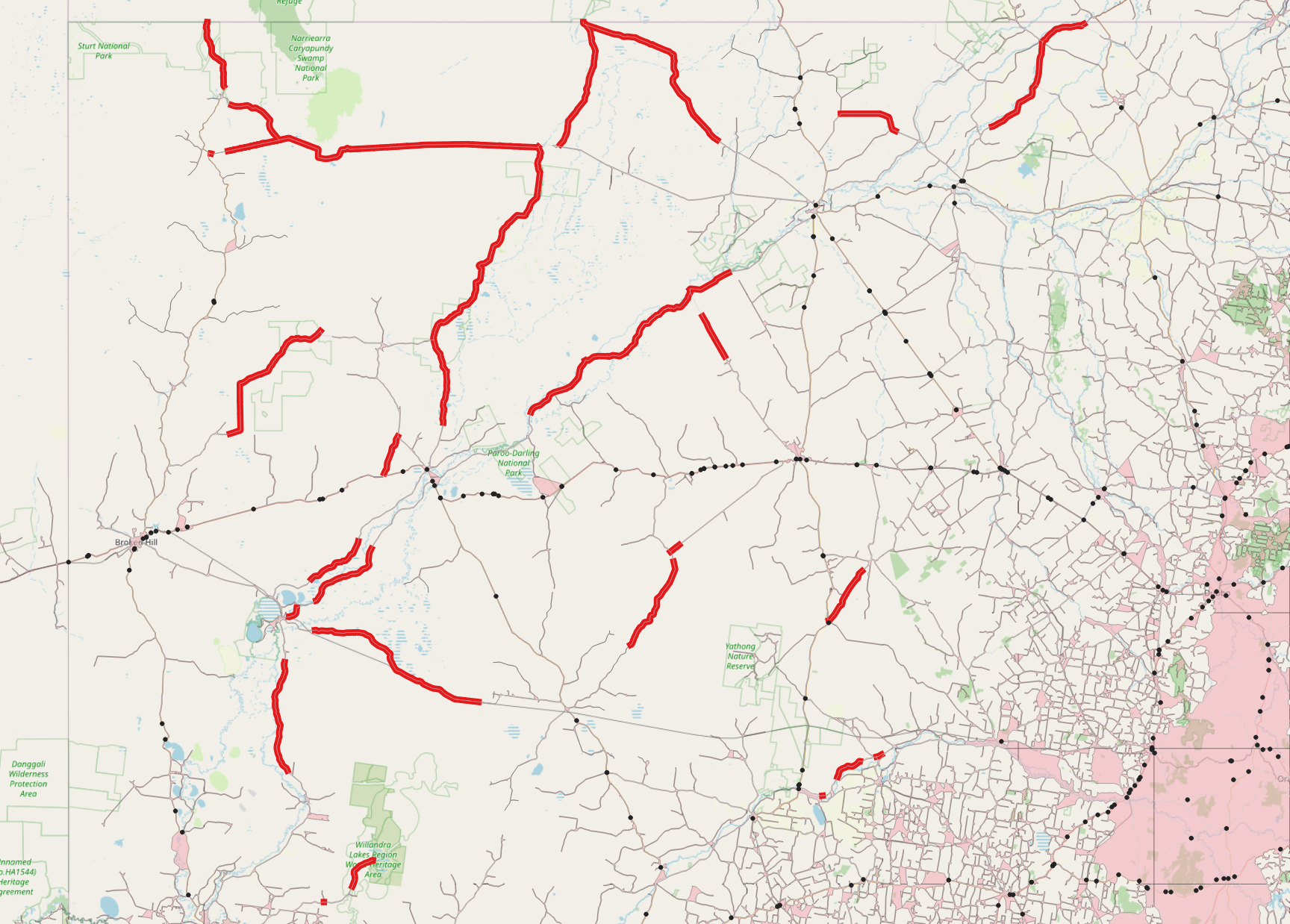
All highways more than 2 hours from a rest stop are located in the north-west of NSW. That said, many of these ‘highways’ are unsealed roads connecting rural centres but not necessarily on the busiest of routes.
The next stage of the study might be to analyse each of these 34 sections of highway to identify potential rest stops.
The process is not perfect – but a great starting point for discussion.
Final Map
Using QGIS2Web, I created a quick map of the final orphaned segments.
Recent Comments